 Copyright © 2002 AIS at ICS PAS, Warsaw, Poland. All rights reserved.
Information about this page format is available HERE.
Results of experiments disscussed in paper
"Immune Memory Control in Artificial Immune System"
K. Trojanowski, S. T. Wierzchoń, submitted to National Conference on Evolutionary Computation and Global Optimization, 2002.
Page includes detailed graphs of results of experiments refered in the paper.
In our experiments we tested two approaches to memory management problem. In previous research (Trojanowski, Wierzchoń 2002) it was showed, that the presence of memory can improve effciency of the artificial immune system in searching for optima of non-stationary environments, however the main problem was a form of memory control, i.e. memory structure, and rules of remembering, remindind and forgetting. In this study we compare two methods of memory control. In both methods there exists a memory buffer in artificial immune system. The buffer is one and only one, it is common for all individuals in the system and may contain many individuals obtained during the search process. The size of the memory buffer is constant during the time of search.
The two already mentioned methods have different population architectures. In the first one there is one population which exchanges information with memory buffer, and in the second one, there are two populations, which can write to memory but only one of them can read.
Here, the system consists of a population of antibodies, which perform search process over the search space and a memory buffer storing complete individuals remembered during the search. The population is initialised randomly once at the beginning of the search and continues its search after every change in optimised environment without any significant modification of a group of individuals. The only modification performed after change (which represents presentation of another antigen to the immune system) is concerned with exchange of a single individual with the memory buffer.
In this approach there are two population of antibodies: the first one, called population of explorers, represents primary response of an immune system, and the second one, called exploitative population, represents secondary response of the system. There is also a memory buffer, which represents memory cells of the system. This architecture of populations corresponds to the idea proposed by J. Branke (1999).
After every change in the optimised environment, both populations start their search processes in parallel at the same time. The difference is in starting points of these populations. Population of explorers starts with randomly generated and therefore uniformly distributed over the search space population of individuals. Exploitative population takes the best individual form the memory (here "the best" means that all individuals from the memory buffer are re-evaluated with evaluation function after change, and then the best one is selected), and builds its population using this individual as a "seed". All individuals in exploitative population are created by light mutation of the seed. Then the search process starts. During the search process populations do not disturb each other, i.e. do not exchange any information. They just compete in the race to the optimum. Returned value of this searching pair is the better individual of the best individuals of the two populations.
We tested two forms of memory control: for single-population architecture of a system and for double-population architecture. For both of forms, three mechanisms concerned with memory access are discussed: remembering, forgetting and recalling.
A set of experiments was performed. We did three groups of experiments with two types of environments. Our test-bed was a test-case generator proposed by Trojanowski and Michalewicz (1999). The generator creates a convex search space, which is a multidimensional hypercube. It is divided into a number of disjoint subspaces of the same size with defined simple unimodal functions of the same shape but possibly different value of optimum. In case of two-dimensional search space we simply have a patchy landscape, i.e. a chess-board with a hill in the middle of every field. Hills do not move but cyclically change their heights what makes the landscape varying in time. The goal is to find the current highest hill. In our experiments there was a sequence of fields with varying hills' heights. Other fields of the space were static. We did experiments with two-dimensional search space where the chess-boards were of size 4 by 4, i.e. with 16 fields, and of size 6 by 6, i.e. with 36 fields. Thus the search spaces consisted of 15 local optima and one global optimum in the first case, and of 35 local optima and one global optimum in the second one. We tested four shapes of the sequence of non-stationary fields presented in Figure 1. In the figure, values in cells are weights of unimodal fuctions of the respective fields, which control heights of the hills. In other words the function located at the (i,j)-field is of the form fij(x,y) = wij×g(x-ai, y-bj), where g is a fixed unimodal function and (ai, bj) is the center of this field. Lower index at the value in the cell represents the position of the field in the sequence of presented optima. The environments #1 and #3 (left part of Figure 1) were test-beds for experiments with cyclic changes, while the environments #2 and #4 (right part of Figure 1) were test-beds for experiments with both cyclic and acyclic changes. The aim of these experiments was to trace efficiency of primary (acyclic changes) and secondary (cyclic changes) immune response to the antigens (i.e. current optima). For experiments with cyclic changes a single epoch obeys 5 cycles of changes. In all the experiments each antigen has been presented through 10 iterations. Thus, in case of the environment #1 a single epoch took 200 iterations, in case of the environment #2 - 400 iterations, in case of the environment #3 - 300 it-erations, and in case of the environment #4 - 600 iterations. Experiments with non-cyclic changes were based on the environments #2 and #4 and a single epoch included just one cycle of changes and took 80 and 120 iterations respectively.
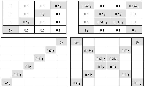
Figure 1. Environments #1 (top left), #2 (top right), #3 (bottom left) and #4 (bottom right) - shapes of the sequence of non-stationary fields in testing environments. Some more figures with 3D visualisation of testing environments available here.
For the six environments described above we did series of experiments with external memory buffer of different sizes - from zero to 50. Every experiment was repeated through 100 epochs and in the later figures we always study average values of these 100 epochs. For the results estimation we used a measure proposed by Trojanowski and Michalewicz (1999): Accuracy. Accuracy is a difference between the value of the current best individual in the population of the "just before the change" generation and the optimum value averaged over the entire run. For this measure the smaller values are the better results.
Obtained values of Accuracy are presented in the figures. In every figure we compare two graphs for the two method described above.
The results of cyclic changes are presented in Figure 2 (env. #1) Figure 3 (env. #2), Figure 4 (env. #3), and Figure 5 (env. #4).
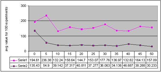
Figure 2. Results for experiments with 11 sizes of memory buffer (from 0 to 50) performed with two methods: single-population (Serie 1) and double-population (Serie 2) approach for environment #1 (cyclic changes). More detailed figures of the results - here
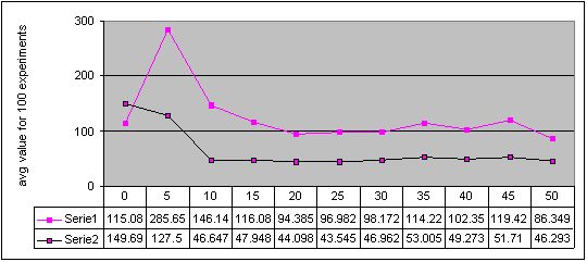
Figure 3. Results for experiments with 11 sizes of memory buffer (from 0 to 50) performed with two methods: single-population (Serie 1) and double-population (Serie 2) approach for environment #2 (cyclic changes). More detailed figures of the results - here
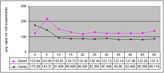
Figure 4. Results for experiments with 11 sizes of memory buffer (from 0 to 50) performed with two methods: single-population (Serie 1) and double-population (Serie 2) approach for environment #3 (cyclic changes). More detailed figures of the results - here
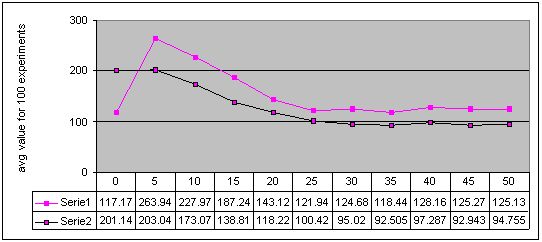
Figure 5. Results for experiments with 11 sizes of memory buffer (from 0 to 50) performed with two methods: single-population (Serie 1) and double-population (Serie 2) approach for environment #4 (cyclic changes). More detailed figures of the results - here
The results of cyclic changes are presented in Figure 6 (env. #2) and Figure 7 (env. #4).
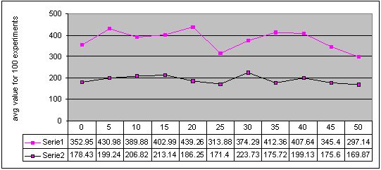
Figure 6. Results for experiments with 11 sizes of memory buffer (from 0 to 50) performed with two methods: single-population (Serie 1) and double-population (Serie 2) approach for environment #2 (non-cyclic changes). More detailed figures of the results - here
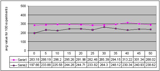
Figure 7. Results for experiments with 11 sizes of memory buffer (from 0 to 50) performed with two methods: single-population (Serie 1) and double-population (Serie 2) approach for environment #4 (non-cyclic changes). More detailed figures of the results - here
Results obtained for the single-population approach applied to cyclically changing environments show, that too small memory buffer can significantly decrease quality of obtained results. When the memory buffer is large enough, obtained results become as good as the results without memory or even slightly better, but in general it is easy to come to convinction that memory cannot help much with non-stationary optimisation process.
Completely different results were obtained for experiments with cyclically changing environments and with the double-population approach. We can see that artificial immune system with even small memory buffer is better than the pure system. However, every type of changes in the environment has a kind of limes in memory buffer size, such that for algorithms with larger memory buffer, obtained results are almost the same while the computation cost is obviously higher. The value of this limes, i.e. optimal memory buffer size is the most probably concerned with a length of a cycle of changes. This conclusion can be confirmed by observation that for environment with a cycle of changes of length 12, the results stopped to be improved for memory buffer of size 30 (Figure 5) while for a cycle of changes of length 6 - for memory buffer of size 15 (Figure 4). However, a shape of a path of changes should be also taken into account in this considerations (compare also Figures 2 and 3).
Experiments with cyclically changing environment showed that the form of memory control plays key role in efficiency of the artificial immune system, and forces a form of architecture of populations in the system.
For experiments with non-cyclically changing environments, both approaches did not improve obtained results too much and sometimes even decreased their quality. Obtained graphs (Figures 6 and 7) show that differences between results for experiments with and without memory are not significant and do not show any dependency between memory buffer size and quality of obtained results.
Finally, we can also see, that in three of four environments with cyclic changes, the better results were obtained when algorithm continued search after change with the same population, as before the change. The results were worse when algorithm every time started from scratch (see Figures 2, 3, 4 and 5 - accuracy values for experiments with memory buffer of size zero).
Copyright © 2002 AIS at ICS PAS, Warsaw, Poland. All rights reserved.
Information about this page format is available HERE.