 Copyright © 2002 AIS at ICS PAS, Warsaw, Poland. All rights reserved.
Information about this page format is available HERE.
Results of experiments disscussed in paper
"Memory Management in Artificial Immune System"
K. Trojanowski, S. T. Wierzchoń, submitted to
International Conference on Neural Nets and Soft Computing, 2002.
Page includes graphs of results of experiments refered in the paper but not included in its final version because of page number limitation.
We performed a set of experiments with the algorithm described in previous section. We did three groups of experiments with two types of environments. Our test-bed was a test-case generator proposed by Trojanowski and Michalewicz (1999). The generator creates a convex search space, which is a multidimensional hypercube. It is divided into a number of disjoint subspaces of the same size with defined simple unimodal functions of the same shape but possibly different value of optimum. In case of two-dimensional search space we simply have a patchy landscape, i.e. a chess-board with a hill in the middle of every field. Hills do not move but cyclically change their heights what makes the landscape varying in time. The goal is to find the current highest hill. In our experiments there was a sequence of fields with varying hills' heights. Other fields of the space were static. We did experiments with two-dimensional search space where the chess-boards were of size 4 by 4, i.e. with 16 fields, and of size 6 by 6, i.e. with 36 fields. Thus the search spaces consisted of 15 local optima and one global optimum in the first case, and of 35 local optima and one global optimum in the second one. We tested four shapes of the sequence of non-stationary fields presented in Figure 2. In the figure, values in cells are weights of unimodal fuctions of the respective fields, which control heights of the hills. In other words the function located at the (i,j)-field is of the form fij(x,y) = wij×g(x-ai, y-bj), where g is a fixed unimodal function and (ai, bj) is the center of this field. Lower index at the value in the cell represents the position of the field in the sequence of presented optima. The environments #1 and #3 (left part of Figure 2) were test-beds for experiments with cyclic changes, while the environments #2 and #4 (right part of Figure 2) were test-beds for experiments with both cyclic and acyclic changes. The aim of these experiments was to trace efficiency of primary (acyclic changes) and secondary (cyclic changes) immune response to the antigens (i.e. current optima). For experiments with cyclic changes a single epoch obeys 5 cycles of changes. In all the experiments each antigen has been presented through 10 iterations. Thus, in case of the environment #1 a single epoch took 200 iterations, in case of the environment #2 - 400 iterations, in case of the environment #3 - 300 it-erations, and in case of the environment #4 - 600 iterations. Experiments with non-cyclic changes were based on the environments #2 and #4 and a single epoch included just one cycle of changes and took 80 and 120 iterations respectively.
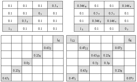
Figure 2. Environments #1 (top left), #2 (top right), #3 (bottom left) and #4 (bottom right) - shapes of the sequence of non-stationary fields in testing environments. Some more figures with 3D visualisation of testing environments available here.
For the six environments described above we did series of experiments by changing the parameters n (step 2 of the algorithm in Figure 1) - see Figure 4.
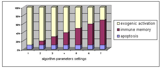
Figure 3. Division of population into activated individuals and individuals for apoptosis. Individuals that do not belong to any of the two subgroups are supposed to be an immune memory structure.
Every experiment of the seven from the Figure 3 was repeated through 200 epochs and in the later figures we always study average values of these 200 epochs. For the results estimation we used two measures proposed by Trojanowski and Michalewicz (1999): Accuracy and Adaptability. Accuracy is a difference between the value of the current best individual in the population of the "just before the change" generation and the optimum value averaged over the entire run. Adaptability is a difference between the value of the current best individual of each generation and the optimum value averaged over the entire run. For both measures the smaller values are the better results.
The results of cyclic changes are presented in Figure 4 (env. #1) Figure 5 (env. #2), Figure 6 (env. #3), and Figure 7 (env. #4).

Figure 4. Results for experiments with 7 types of parameter settings and three types of memory management performed with environment #1 (cyclic changes).
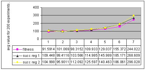
Figure 5. Results for experiments with 7 types of parameter settings and three types of memory management performed with environment #2 (cyclic changes).

Figure 6. Results for experiments with 7 types of parameter settings and three types of memory management performed with environment #3 (cyclic changes).
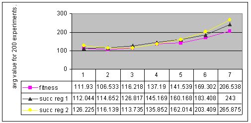
Figure 7. Results for experiments with 7 types of parameter settings and three types of memory management performed with environment #4 (cyclic changes).
Results of experiments with cyclic changes showed, that none of tested memory management techniques was 100% successful in giving the better results. For different types of environments, different strategies won in this competition.
The results of cyclic changes are presented in Figure 8 (env. #2) and Figure 9 (env. #4).
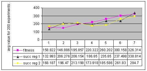
Figure 8. Results for experiments with 7 types of parameter settings and three types of memory management performed with environment #2 (non-cyclic changes).
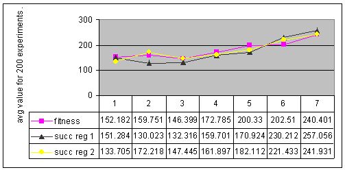
Figure 9. Results for experiments with 7 types of parameter settings and three types of memory management performed with environment #4 (non-cyclic changes).
Results of experiments with non-cyclic changes also showed, that none of tested memory management techniques was 100% successful in giving the better results.
Although for different types of environments, different strategies won the competition, presence of memory - i.e. of a group of individuals in a gap between the group of stimulated and deleted antibodies (defined in Figure 3) - does not guarantee conclusively better results, than in case where the gap is empty (i.e. in the first setting of the parameters). Table 1 summarizes the cases, where memory improved the algorithm.
| method vs. environment | #1 cyclic | #2 cyclic | #3 cyclic | #4 cyclic | #2 non-cyclic | #4 non-cyclic |
|---|---|---|---|---|---|---|
| fitness | No | No | No | Yes | Yes | Yes |
| success reg. (1) | Yes | Yes | Yes | No | No | Yes |
| success reg. (2) | No | Yes | Yes | Yes | No | No |
Table 1. Table of cases, where presence of memory gave better results, than its absence.
Number of cases, where memory improved algorithm results is just a little bigger, than the number of cases, where the results got decreased. That observation indicates, that: (a) the memory emerges indeed, (b) it improves algorithm behaviour, but current form of its management is rather insufficient. In further research we will work on searching other methods of memory management, more resistant to side effects of exogenic activation and apoptosis that corrupt memory content.
Copyright © 2002 AIS at ICS PAS, Warsaw, Poland. All rights reserved.
Information about this page format is available HERE.